You ask a chatbot to explain an invoice. It writes fluent English, recognises the supplier and suggests a follow-up question. What actually happened? Did it look up a rule, remember a document, learn from your message, or calculate an answer?
Those are different mechanisms. Understanding the difference is the first step toward using AI well.
This guide starts with a small prediction problem and builds toward modern language models. You need no previous AI knowledge. The mathematics is explained in words, and the optional Python experiments run on an ordinary computer without a GPU, an account or paid API access. We will train a real, very small neural network and inspect language-model building blocks. We will not pretend that a classroom experiment reproduces an industrial LLM.
Research checked: 20 October 2026. The fundamentals below are longstanding. Section 19 separately examines recent developments and distinguishes published research claims from the measurements in our own examples.
Reading route: The terminology · Inside a neuron · Train a network · Language and tokens · Transformers · RAG and fine-tuning · Current research · Model metrics · Beginner questions.
1. The map: AI, machine learning, neural networks and LLMs
Artificial intelligence (AI) is the broad field of building systems that perform tasks associated with intelligence: recognising patterns, planning, interpreting language or making decisions. An AI system can use explicit rules, search, optimisation, learned models, or a combination.
Machine learning (ML) develops models whose behaviour is fitted from examples. Instead of writing every decision rule ourselves, we choose a model structure and a learning procedure that adjusts its parameters using data. Google's Machine Learning Crash Course provides a useful introductory route through this field.
A neural network is one family of ML models. It connects numerical operations in layers and learns adjustable weights. Deep learning uses neural networks with multiple representation-learning layers. There is no universal layer-count threshold that makes a model “deep.”
A language model assigns probabilities to tokens or token sequences. A large language model (LLM) is a large learned language model, usually based on a deep neural network. “Large” has no permanent minimum parameter count. A model that looked enormous a decade ago might be small by today's standards; see the LLM research survey for the broader development of the field.
Generative AI produces content such as text, images or audio. Its scope overlaps these categories: a language model can generate text, but an image generator need not be an LLM. An AI agent is an application that uses a model within a loop to pursue a task, often with tools and external state. An agent is a system design, rather than a new synonym for a neural network.
| Term | What it describes | Example |
|---|---|---|
| AI | The broad field | A planning system combining search and rules |
| ML | Fitting behaviour from data | Predicting whether a support ticket is urgent |
| Neural network | A parameterised model family | Layers learning nonlinear combinations of inputs |
| Deep learning | Learning through multiple neural layers | Image recognition with learned representations |
| Language model | A probability model over language tokens | Predicting a likely continuation |
| LLM | A large neural language model | A model generating a technical explanation |
| Agent | An application with model-directed task steps | Searching approved documents before drafting a reply |
The last row describes how a model is used. It should not be drawn as another mathematical subset inside the LLM category.
2. What “learning from data” means
Imagine a fictional service desk. For each historical support ticket we record the number of affected users and how long the service has been unavailable. A reviewer has labelled the ticket “urgent” or “not urgent.”
Each ticket is an example. Its measurable inputs are features. The reviewer's answer is the label or target. The collection is a dataset. The fitted numerical function is the model.
Our model might calculate a score from the two features. During training, we compare its score with the target and adjust its parameters to reduce the error. Later, we supply the features of a new ticket and calculate a prediction. That later calculation is inference.
This fictional example also reveals the limits. If reviewers used inconsistent definitions of urgency, the model receives inconsistent targets. If the dataset excludes weekend outages, weekend behaviour is uncertain. If a contract has changed, historical labels may encode an obsolete policy. Collecting more rows does not automatically fix any of these problems.
There are several common learning setups:
- Supervised learning: learn from inputs paired with targets, such as tickets and urgency labels.
- Unsupervised learning: discover structure without a supplied target for every example, such as grouping similar tickets.
- Self-supervised learning: derive training targets from the data itself. In a text sequence, earlier tokens can be inputs and the next token the target.
- Reinforcement learning: learn a policy using rewards associated with actions and their consequences. A reward is a training signal, not proof that an action is correct or safe.
Self-supervision is often grouped under unsupervised learning, but its prediction task has explicit targets. “No one manually labelled every word” does not mean “there was no target.” The introductory LLM module helps connect language modelling with the wider ML landscape.
3. Prediction problems are not all the same
Regression predicts a numerical quantity: perhaps the duration of an outage. Classification selects a category: urgent or not urgent. Clustering groups examples by a similarity criterion. Generation produces a structured output, such as a sequence of words.
For a simple regression example, imagine predicting electricity use from opening hours. A linear model could be written as prediction = weight × hours + bias. The weight controls the slope; the bias shifts the line. Both are learned parameters. The linear regression chapter in Dive into Deep Learning explains how such a prediction function connects to an error measure.
Suppose the weight is 2 and the bias is 3. For 4 opening hours, the prediction is 11 units. If the observed value is 13, the error is −2 and its square is 4. Averaging squared errors across examples gives mean squared error, one possible loss function.
That arithmetic does not establish a causal relationship. Hours and consumption might both depend on production volume. An accurate prediction alone does not tell us what would happen if we intervened and changed the opening hours.
A neural network is not automatically the best solution. A rule is appropriate for a fixed contractual requirement. A linear model can be an effective baseline. Trees and boosted trees deserve consideration for structured tables. The sensible starting point is the task and its evidence, not the most elaborate model name.
4. A neuron is a calculation
An artificial neuron takes numbers, multiplies them by weights, adds them, adds a bias, and applies an activation function. For two inputs:
z = w₁x₁ + w₂x₂ + b, followed by output = activation(z).
For example, let the inputs be 2 and 3, the weights 0.5 and −1, and the bias 1. Then z = 1 − 3 + 1 = −1. A ReLU activation returns max(0, z), so this neuron's output is 0. With a sigmoid activation, the output would be about 0.269.
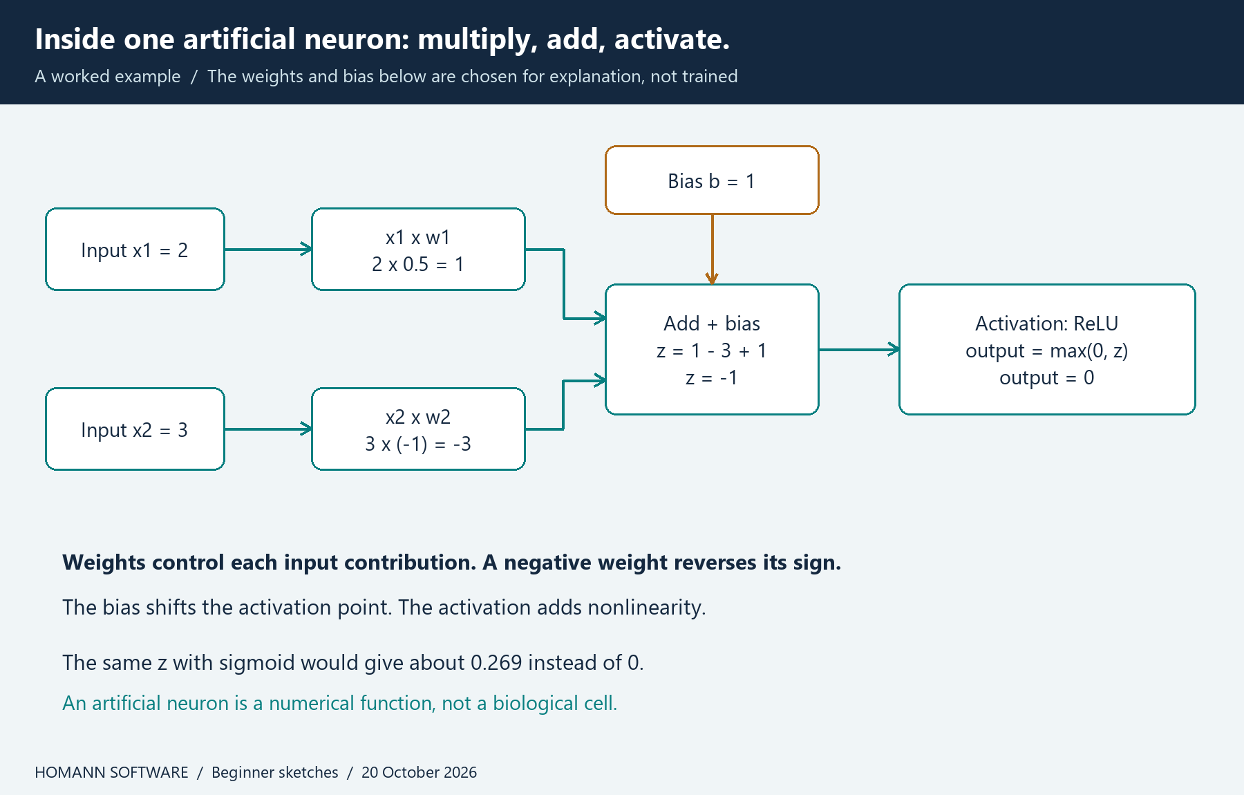
Figure 1. Follow one neuron from left to right: multiply each input by its weight, add the contributions and bias, then apply the activation. The values are chosen to explain the calculation.
These are mathematical units. Biological neurons inspired some early terminology, but an artificial network is not a detailed simulation of a human brain.
The nonlinearity matters. Composing affine transformations without a nonlinear activation still produces an affine transformation. With suitable nonlinear layers, a network can represent patterns that one linear boundary cannot. The multilayer perceptron chapter develops this distinction.
Useful activations include ReLU, which clips negative inputs to zero; tanh, which maps into the range −1 to 1; and sigmoid, which maps finite real inputs into values between 0 and 1. Choosing an activation depends on its role. Modern networks often use other functions in hidden layers. A binary classifier may use sigmoid for its final score, while a multiclass classifier commonly uses softmax across class logits.
An input layer receives features, hidden layers transform representations, and an output layer produces the task's prediction. The word “hidden” means the internal representation is not itself the supplied target. It does not mean that its numbers are inaccessible.
The next sketch shows how neurons work together. It deliberately uses a separate, hand-configured network so that every number fits on the page. Both hidden neurons receive the same inputs, 2 and 3, but use different weights and biases. Their outputs are 0 and 2.5. A linear output neuron combines those values into 0.4 × 0 + 0.8 × 2.5 + 0.1 = 2.1.
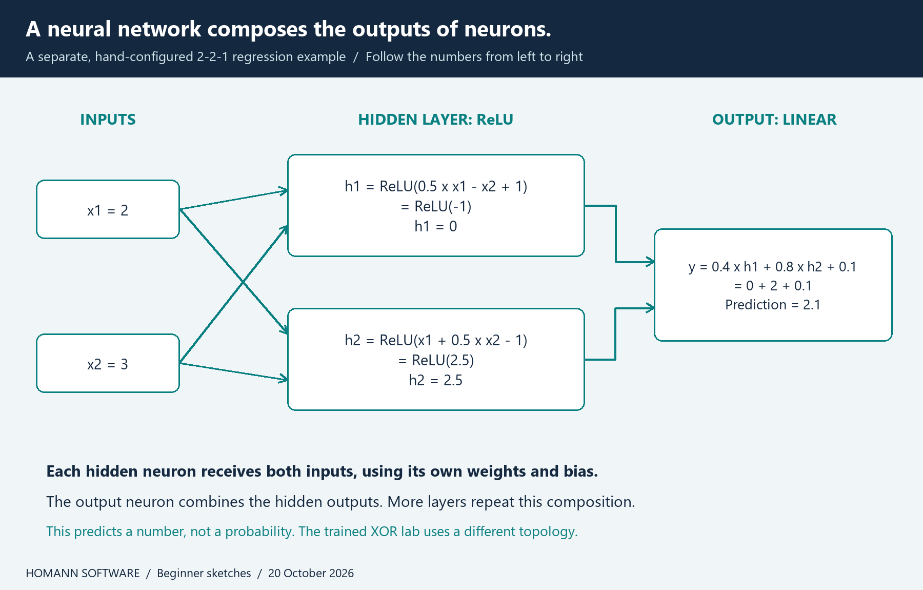
Figure 2. A network composes several neuron calculations. These illustrative weights are chosen, not learned; this regression example is different from the trained XOR classifier in section 6.
This is the general forward-pass idea: one layer's outputs become the next layer's inputs. The structure specifies which computations are connected; the weights and biases specify their current numerical behaviour. Training adjusts those parameters. Simply drawing more connections does not make the network learn.
5. How a network learns: forward pass, loss and backward pass
Training repeatedly performs a few concrete operations.
First, a forward pass calculates the prediction using the current parameters. Second, the loss measures how that prediction differs from the training target. Third, backpropagation applies the chain rule from calculus to compute how the loss changes with each parameter. Fourth, an optimiser uses those gradients to update the parameters. Backpropagation computes derivatives; the optimiser determines the update. These are separate responsibilities, as explained in the forward and backward propagation chapter.
In basic gradient descent, the update is:
new weight = old weight − learning rate × loss gradient.
The gradient points in the local direction of increasing loss. Subtracting a small multiple of it attempts to move downhill. It does not guarantee that every step improves the loss or that a globally best solution will be found. The gradient descent chapter explains why step size and the shape of the objective matter.
Consider a single weight of 0.5, a gradient of 0.2 and a learning rate of 0.1. The update produces 0.48. A negative gradient would increase the weight instead. In a large network, the same principle operates over arrays containing many parameters.
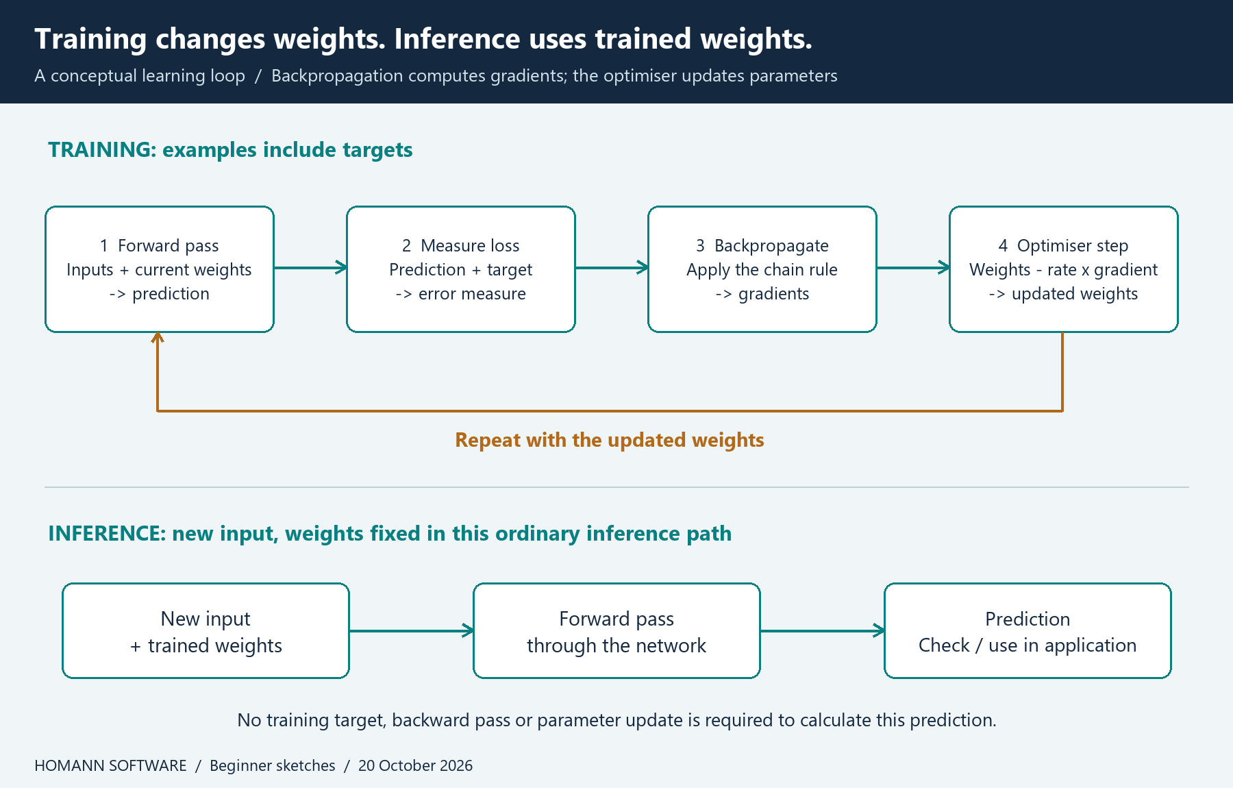
Figure 3. During training, the loss connects predictions to targets and gradients guide parameter updates. Ordinary inference uses the fitted weights to calculate a prediction; it does not require a training target or a parameter update.
An epoch means one pass through the training data. A batch is the group of examples used to compute an update. A training step is one update. Our example uses the complete four-example dataset for every step, so each step also covers one epoch. That equivalence does not hold when an epoch contains many minibatches.
Parameters are the weights and biases learned by the procedure. Hyperparameters are choices such as learning rate, hidden-layer size and training duration. They are normally chosen using validation evidence. Giving a model more parameters can increase its capacity, but capacity is different from evidence that it learned the right pattern.
6. A runnable neural network you can inspect
XOR is a small classification problem. Its output is 1 when two binary inputs differ and 0 when they match:
| First input | Second input | Target |
|---|---|---|
| 0 | 0 | 0 |
| 0 | 1 | 1 |
| 1 | 0 | 1 |
| 1 | 1 | 0 |
On a square, the positive examples occupy opposite corners. A single straight boundary cannot separate the two classes. A hidden layer with nonlinear activations can construct a suitable representation.
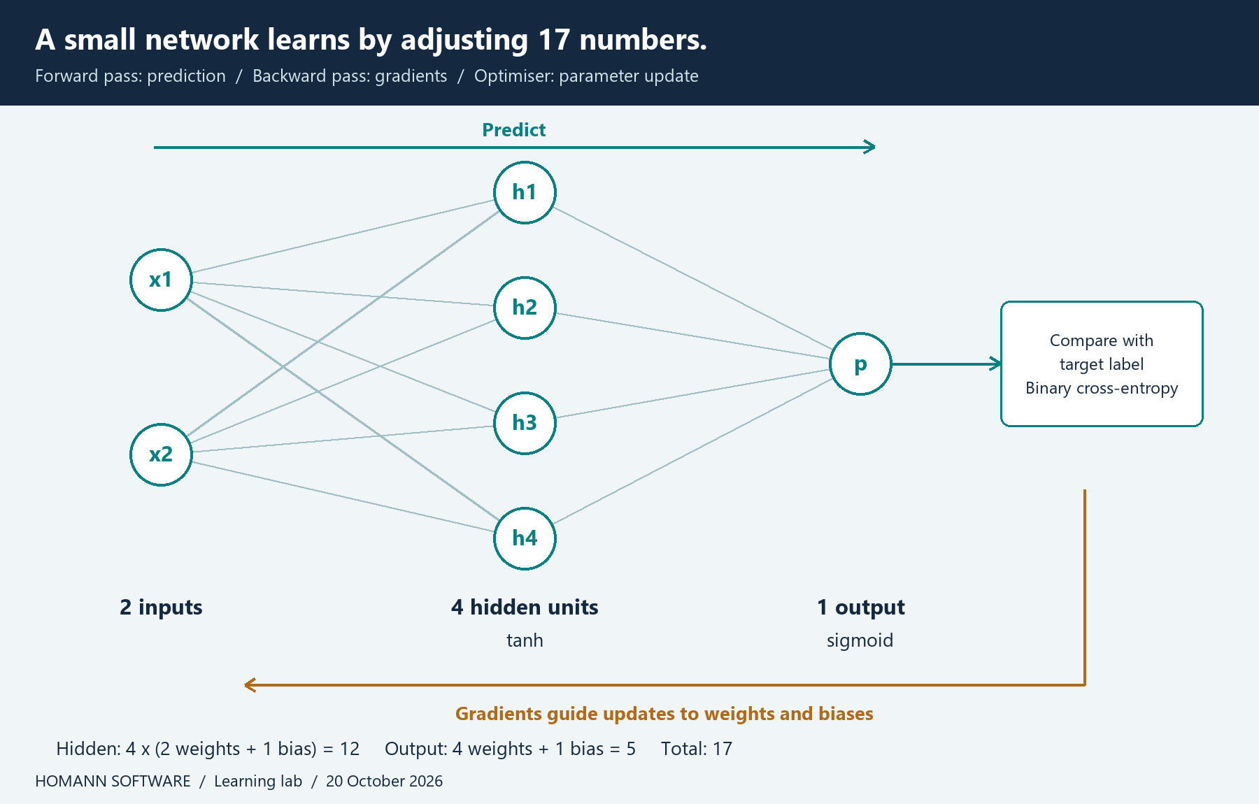
Figure 4. The exact 2–4–1 topology used in our experiment. Seventeen adjustable parameters connect prediction, loss and gradient updates.
The complete file below uses only Python's standard library. Four hidden units each have two input weights and one bias: 4 × 3 = 12 parameters. The output has four weights and one bias, giving 17 parameters in total. Hidden units use tanh; the output uses sigmoid. Training minimises mean binary cross-entropy with full-batch gradient descent.
Binary cross-entropy penalises assigning low probability to the correct binary target. Its derivative with respect to the sigmoid input logit simplifies to predicted score − target. For tanh, the local derivative is 1 − hidden output². Those two identities explain the handwritten gradient calculation in the code. The loss is computed directly from logits using a numerically stable expression, rather than taking the logarithm of a rounded probability.
Save this as neural_net.py:
"""A 2-4-1 neural network, handwritten gradients, standard library only."""
import math
import random

XOR = [((0.0, 0.0), 0.0), ((0.0, 1.0), 1.0),
       ((1.0, 0.0), 1.0), ((1.0, 1.0), 0.0)]


def sigmoid(z):
    if z >= 0:
        return 1.0 / (1.0 + math.exp(-z))
    e = math.exp(z)
    return e / (1.0 + e)


class TinyNet:
    # Four hidden units: each has two input weights and one bias.
    # Output: four weights and one bias. Total: 17 parameters.
    def __init__(self, seed=7):
        rng = random.Random(seed)
        self.p = [rng.uniform(-1.0, 1.0) for _ in range(17)]

    def forward(self, x):
        if len(x) != 2 or not all(math.isfinite(v) for v in x):
            raise ValueError("expected two finite input numbers")
        h = [math.tanh(self.p[3*j]*x[0] + self.p[3*j+1]*x[1]
                       + self.p[3*j+2]) for j in range(4)]
        z = sum(self.p[12+j]*h[j] for j in range(4)) + self.p[16]
        return h, z, sigmoid(z)

    def loss_and_grad(self, data):
        if not data:
            raise ValueError("data must not be empty")
        g, loss = [0.0]*17, 0.0
        for x, y in data:
            if y not in (0.0, 1.0):
                raise ValueError("binary labels required")
            h, z, prob = self.forward(x)
            # Stable binary cross-entropy from the logit.
            loss += max(z, 0.0) - y*z + math.log1p(math.exp(-abs(z)))
            dz = prob - y
            for j in range(4):
                g[12+j] += dz*h[j]
                dh = dz*self.p[12+j]*(1.0 - h[j]*h[j])
                g[3*j] += dh*x[0]
                g[3*j+1] += dh*x[1]
                g[3*j+2] += dh
            g[16] += dz
        n = len(data)
        return loss/n, [v/n for v in g]

    def fit(self, data, steps=10000, learning_rate=0.2):
        if steps < 1 or not math.isfinite(learning_rate) or learning_rate <= 0:
            raise ValueError("positive steps and finite learning rate required")
        initial, _ = self.loss_and_grad(data)
        for _ in range(steps):
            _, g = self.loss_and_grad(data)
            self.p = [p - learning_rate*dg for p, dg in zip(self.p, g)]
        final, _ = self.loss_and_grad(data)
        return initial, final


if __name__ == "__main__":
    net = TinyNet()
    initial, final = net.fit(XOR)
    print(f"Mean training BCE: {initial:.6f} -> {final:.6f}")
    for x, y in XOR:
        prob = net.forward(x)[2]
        print(f"{x}: target={int(y)} score={prob:.6f} class={int(prob >= 0.5)}")
Run it with:
python neural_net.py
The executed result on Python 3.12.14 was:
Mean training BCE: 0.815205 -> 0.003430
(0.0, 0.0): target=0 score=0.001165 class=0
(0.0, 1.0): target=1 score=0.997289 class=1
(1.0, 0.0): target=1 score=0.995591 class=1
(1.0, 1.0): target=0 score=0.005408 class=0
The network fitted all four training cases. Its output scores are not independently calibrated probabilities about business events. We deliberately used the entire XOR truth table to make optimisation visible. There is no independent test set here, and this result makes no claim about generalisation, production quality or the capabilities of an LLM.
The downloadable test suite checks every analytical gradient against a central finite difference: change one parameter slightly upward and downward, observe the two losses, and divide their difference by twice the perturbation. That provides an independent numerical check on the derivative implementation. The tests also check the final fit, averaging, extreme logits and invalid inputs.
7. Learning the training data is not enough
A network can perform well on examples it has seen and fail on new ones. Overfitting means fitting peculiarities of the training data too closely for the intended task. Underfitting means the model or training procedure fails to capture useful structure even in the available data.
Use different data for different decisions:
- Training set: fit parameters.
- Validation set: choose configurations, thresholds and other development decisions.
- Test set: estimate performance after those choices are fixed.
Repeatedly tuning against a test score turns the test set into another development set. There is no universally correct 80/20 or 70/15/15 split; the sizes must support the actual measurement. Google's dataset splitting guidance explains these roles and the danger of repeated reuse.
Data leakage occurs when training or development uses information that would not be available under the intended prediction conditions. A ticket's final resolution time, for example, cannot be a legitimate input when predicting urgency at creation. Duplicate tickets or multiple records from one incident can also create misleadingly easy evaluation if they appear on both sides of a split.
Fit scaling and other learned preprocessing on the training partition, then apply that fitted transformation to validation and test data. Scikit-learn's common pitfalls guide shows why preprocessing before the split can leak information. For future predictions, a chronological split is often more realistic; related users, customers or incidents may require group-based separation.
Ways to control overfitting include collecting more representative data, simplifying the model, penalising excessively large weights, and stopping training based on validation performance. None can repair a target that measures the wrong business outcome. A model that predicts whether a reviewer clicked “urgent” may be learning review habits rather than actual service impact.
8. What should we measure?
Consider a deliberately fictional evaluation of 1,000 tickets. Only 20 are truly urgent. A classifier that always says “not urgent” achieves 98% accuracy while finding none of the urgent cases.
Now suppose another classifier flags 30 tickets. Fifteen are truly urgent, fifteen are false alarms, and five urgent tickets are missed. Its precision is 15/30 = 50%: half of its alerts are correct. Its recall is 15/20 = 75%: it finds three quarters of the urgent cases. Its accuracy is (15 + 965)/1,000 = 98%. The two classifiers share the same accuracy and have very different usefulness.
Google's classification metrics reference defines these quantities and explains the role of thresholds. A higher alert threshold may reduce false alarms while missing more incidents. Choose that trade-off using the cost of the errors and validation evidence.
For our fictional support desk, a useful acceptance condition could include missed critical incidents, reviewer workload, response time and performance across customer groups. That is a proposed evaluation design, not an adopted Homann policy or a measured result.
Unit tests answer whether software behaves as specified. Statistical evaluation asks how a fitted model performs on a relevant sample. Operational monitoring asks what happens after deployment. A robust AI application needs all three; passing the Python tests in this article only addresses the first, plus the explicitly reported toy-training result.
9. From numbers to language: tokens and embeddings
Computers do not feed raw words into a neural layer. A tokeniser maps text into token IDs. Tokens may represent words, word fragments, punctuation, characters or byte-derived pieces, depending on the tokeniser. Do not assume that one word equals one token, or that English token estimates transfer unchanged to other languages. Google's LLM architecture introduction explains the connection between tokens and language-model inputs.
An embedding maps an ID to a vector: an ordered list of learned numbers. A token ID is a lookup index, not a meaningful numerical magnitude. Token 200 is not automatically twice as meaningful as token 100. The vector gives the network a representation it can transform and compare.
Imagine a deliberately invented two-dimensional space for support topics. “Invoice” might map to [0.8, 0.2] and “payment” to [0.7, 0.3]. Their proximity illustrates learned similarity; these particular numbers are fictional. Actual embeddings usually have many dimensions, and individual coordinates generally do not have simple human labels. Google's embedding-space lesson explains the underlying idea.
A model may begin with a static embedding lookup, then calculate contextual representations in subsequent layers. The word “bank” in a river description should be represented differently from “bank” in a payment request. Sentence and document embeddings used for search are another application; they are not necessarily the same vectors used inside a generative model.
Token order matters too. Transformers incorporate positional information so that rearranging a sequence changes its interpretation. “The customer paid the supplier” and “The supplier paid the customer” contain the same words but describe different events.
10. What language modelling actually predicts
An autoregressive language model estimates the probability of the next token given earlier tokens. Repeating that operation gives a sequence probability:
P(t₁, …, tₙ) = P(t₁) × P(t₂ | t₁) × … × P(tₙ | t₁, …, tₙ₋₁).
The vertical bar means “given.” The formula is a chain of conditional probabilities. A model supplies estimates for the factors. Predicting a rich distribution over continuations can require learning substantial regularities in language, code and descriptions of the world; “next-token prediction” does not imply that the resulting behaviour is trivial. The GPT-3 paper is an influential demonstration of scaling autoregressive language modelling and using examples in context.
During common causal-language-model pretraining, the targets come from the next tokens in the training sequence. A model can predict many training positions in parallel because a causal mask prevents each position from using its future. Generating a continuation is ordinarily sequential: choose a token, append it, and calculate the next distribution.
A tiny bigram model makes conditional prediction easy to inspect. It uses only the previous token. In our three-sentence training corpus, “the cat” occurs twice and “the dog” once. With add-one smoothing over six possible output tokens, the probability after “the” becomes 3/9 for “cat” and 2/9 for “dog.” Each other output gets 1/9.
Smoothing prevents zero probabilities for unseen continuations within that vocabulary. It does not create understanding. Our whitespace tokeniser, fixed vocabulary and one-token context are deliberate simplifications. This count-based model is not a neural network and not an LLM. It is a microscope for one idea shared with more powerful models: conditional next-token probabilities.
11. Transformers and attention, without the mystique
The 2017 Transformer paper, Attention Is All You Need, introduced an architecture built around attention rather than recurrence. Modern conversational models often use decoder-only Transformer variants. Encoder-only and encoder–decoder architectures also serve important purposes; not every language model uses the same layout.
An attention head forms three learned projections of representations: queries (Q), keys (K) and values (V). For each query, dot products with keys produce compatibility scores. Scaling and softmax turn these into nonnegative weights that sum to one. The head then combines value vectors using those weights:
Attention(Q, K, V) = softmax(QKᵀ / √dₖ + mask) V.
Here dₖ is the key/query width. A causal mask excludes future positions. The first position can use itself, the second can use the first two, and so on. Attention is a learned routing-and-mixing calculation, not a guarantee of human-style comprehension or an explanation of a model's complete reasoning.
Multiple heads offer multiple learned projections. Transformer blocks also contain feed-forward networks, residual connections and normalisation. Repeating blocks transforms the representations before an output projection produces vocabulary scores, called logits. Positional information is required because ordinary attention alone does not encode sequence order. The LLM survey discusses the broader architecture and training choices.
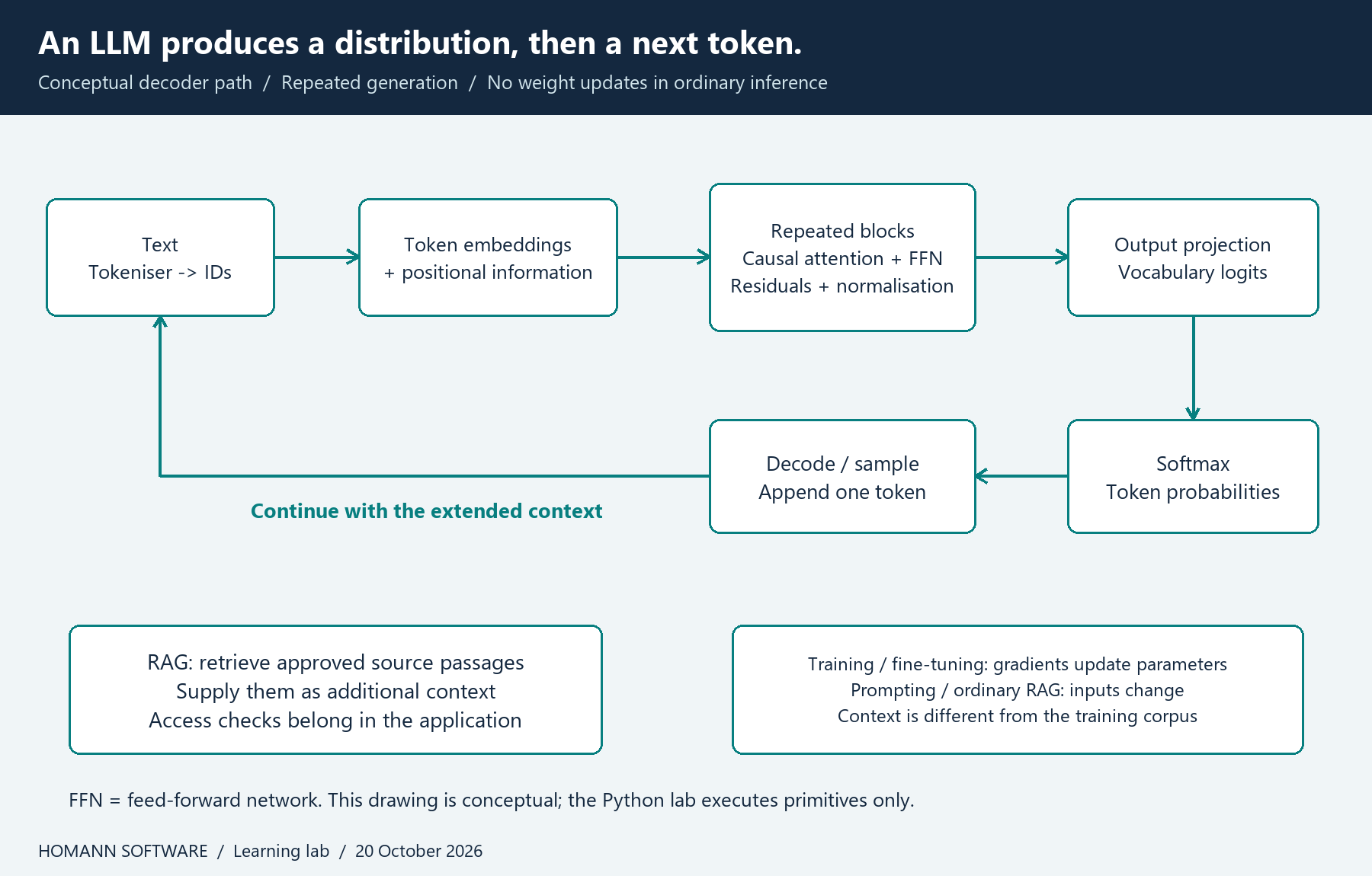
Figure 5. A conceptual token-generation path. Retrieval supplies context around the model; ordinary prompting and retrieval do not update its trained weights.
Our second complete Python file exposes attention directly. The caller supplies Q, K and V; there are no learned projection matrices, Transformer blocks, positional embeddings, automatic differentiation or LLM training. This makes the mask and weighted combination visible while keeping the scope honest.
Save it as language_lab.py:
"""Inspectable language-model primitives; this is NOT a trained LLM."""
from collections import Counter, defaultdict
import math


def softmax(logits, temperature=1.0):
    if (not logits or not math.isfinite(temperature) or temperature <= 0
            or not all(math.isfinite(x) for x in logits)):
        raise ValueError("finite logits and positive finite temperature required")
    # Subtract BEFORE dividing: stable for very small positive temperatures.
    maximum = max(logits)
    exp = [math.exp((x-maximum)/temperature) for x in logits]
    total = sum(exp)
    return [x/total for x in exp]


def attention(q, k, v):
    # One head, causal self-attention; q, k and v supplied directly.
    n = len(q)
    if not n or len(k) != n or len(v) != n:
        raise ValueError("matching nonempty sequence lengths required")
    dk, dv = len(q[0]), len(v[0])
    if (not dk or not dv or any(len(r) != dk for r in q+k)
            or any(len(r) != dv for r in v)
            or not all(math.isfinite(x) for r in q+k+v for x in r)):
        raise ValueError("finite rectangular matrices with matching Q/K width required")
    weights, output = [], []
    for i in range(n):
        # Future keys are excluded, equivalent to a minus-infinity mask.
        logits = [sum(a*b for a, b in zip(q[i], k[j]))/math.sqrt(dk)
                  for j in range(i+1)]
        row = softmax(logits) + [0.0]*(n-i-1)
        weights.append(row)
        output.append([sum(row[j]*v[j][c] for j in range(n))
                       for c in range(dv)])
    return output, weights


class Bigram:
    # Whitespace tokens and add-one smoothing, deliberately simplified.
    def __init__(self, sentences):
        self.counts = defaultdict(Counter)
        self.vocab = set()
        for text in sentences:
            tokens = text.split()
            if not tokens:
                continue
            self.vocab.update(tokens + ["</s>"])
            for a, b in zip(["<s>"] + tokens, tokens + ["</s>"]):
                self.counts[a][b] += 1
        if not self.vocab:
            raise ValueError("nonempty training text required")

    def distribution(self, previous):
        counts = self.counts.get(previous, Counter())
        total = sum(counts.values()) + len(self.vocab)
        return {w: (counts[w]+1)/total for w in sorted(self.vocab)}


if __name__ == "__main__":
    lm = Bigram(["the cat sleeps", "the cat eats", "the dog sleeps"])
    print("Next token after 'the':", lm.distribution("the"))
    print("Temperature 1.0:", [round(x, 6) for x in softmax([2, 1, 0])])
    print("Temperature 0.5:", [round(x, 6) for x in softmax([2, 1, 0], 0.5)])
    out, weights = attention([[1, 0], [0, 1]], [[1, 0], [0, 1]],
                             [[10, 0], [0, 20]])
    print("Causal weights:", weights)
    print("Attention output:", out)
Run python language_lab.py. The first attention row is [1, 0], so its output is exactly the first value vector, [10, 0]. The second row is approximately [0.330238, 0.669762], producing [3.302385, 13.395231]. Our tests independently verify this weighted sum and prove that changing future inputs does not change the first output position.
For ordinary dense full self-attention, comparing every position with every position creates a quadratic number of pair scores in sequence length. Long contexts therefore have computational costs. Optimised kernels, caching and alternative attention designs change practical memory use and execution; our nested-loop teaching implementation is not a performance model for production inference. The StreamingLLM research is one example of work addressing long-sequence operation.
12. Softmax, temperature and why confidence is easy to misread
Softmax converts logits into a probability distribution by exponentiating and normalising them. We subtract the maximum logit first to avoid unnecessarily large exponentials. This preserves the distribution mathematically.
In our executed example, logits [2, 1, 0] produce probabilities [0.665241, 0.244728, 0.090031] at temperature 1.0. Dividing the relative logits by temperature 0.5 produces [0.866813, 0.117310, 0.015876]. The lower temperature concentrates probability on the highest logit. This is a calculation on three supplied scores, not a measurement of a commercial model.
Generation can choose the highest-probability token, or sample. Other sampling methods can restrict candidates, such as retaining a probability-mass prefix. Temperature changes how tokens are selected from scores; it does not verify facts. A highly probable continuation may still make a false statement. The language-model introduction connects output probabilities with text generation.
In many APIs, temperature zero is implemented as a special decoding mode, often greedy selection. Our mathematical helper intentionally requires a strictly positive temperature. Even greedy decoding is not a universal promise of identical output across different models, serving configurations or software versions.
Do not interpret a generated sentence such as “I am 95% certain” as a calibrated estimate. It is text. Even access to token probabilities would not directly yield the probability that a complete factual answer is correct. That requires task-specific measurement and calibration.
13. Pretraining, post-training and ordinary use
Pretraining builds broad capabilities from a large training corpus. For causal text generation, the central objective is commonly next-token prediction. Other model families use objectives such as masked-token prediction. These should not be conflated: predicting the next token from a prefix and recovering a missing token with both left and right context are different training conditions.
Instruction tuning trains a model on examples of desired input/output behaviour. Preference optimisation uses comparisons or feedback about outputs. The InstructGPT paper describes a prominent combination of supervised fine-tuning and reinforcement learning from human feedback. Direct Preference Optimization illustrates a different way to train from preference comparisons. These are historical primary references, not claims that all current products use an identical pipeline.
Inference applies a trained model. In the ordinary inference path described here, sending a prompt does not run gradient updates on the model's weights. An application may save messages, maintain external memory, or a provider may later use permitted data in a separate training process. Those are additional mechanisms, governed by the actual system and service terms.
A context window is the limited input/output token budget a model supports for an interaction. It is working context, not the model's training corpus. Supplying a long manual does not guarantee that every detail will be used reliably.
A parameter count is also different from a token count. Parameters are learned numbers; tokens are sequence units being processed. Their interaction with training data and compute matters. The Chinchilla study investigated how model size and training-token budgets should be balanced under a compute constraint. Its results are a research finding under specified conditions, not a permanent formula for every application.
14. Prompting, RAG and fine-tuning solve different problems
Suppose our fictional support team needs answers from its current operating manual. There are three distinct approaches:
| Approach | What changes? | A useful starting use case | What it does not establish |
|---|---|---|---|
| Prompting | The supplied instructions and context | Specify the task, format and examples | That the answer is factually correct |
| Retrieval-augmented generation (RAG) | Documents retrieved into context | Answer from current approved material | That retrieval found sufficient evidence |
| Fine-tuning | Model parameters or adapter parameters | Learn a repeated task style or behaviour | That every fact is current or reliably recalled |
In RAG, an application searches a source collection, supplies relevant passages to a model, and asks for an answer grounded in those passages. The original RAG paper combined retrieval with generation for knowledge-intensive tasks. Modern implementations vary. Indexing and retrieving new material is different from updating the generator's weights.
RAG can fail because the source is wrong, the search misses the right passage, permissions are applied incorrectly, or the model misuses the evidence. A citation is useful only if it points to material that actually supports the claim. Access controls belong in retrieval and application design, rather than in a polite instruction asking the model to ignore unauthorised documents.
Fine-tuning changes learned behaviour. Parameter-efficient methods can train a smaller set of additional parameters while keeping most base parameters frozen; LoRA is an influential example. Fine-tuning does not automatically turn weights into an auditable, current document database.
These methods can be combined. A practical experiment might start with prompting, add retrieval for changing reference material, then consider fine-tuning if a measured behavioural gap remains. Evaluate the full system after every material change, including retrieval and the instruction template.
15. Hallucinations, bias and the limits of fluent answers
A language model can produce a plausible unsupported claim, often called a hallucination. Fluency is not an independent fact-checking mechanism. Training objectives, incomplete data, ambiguous prompts and limitations in retrieval or reasoning can all contribute to unreliable outputs.
Evaluation must therefore go beyond whether an answer sounds good. The HELM research advocates measuring multiple dimensions, including accuracy, robustness, calibration, fairness and efficiency, rather than reducing language-model quality to one leaderboard number.
For a fictional support assistant, we could assess whether the cited passage supports each answer, whether it admits missing information, whether it handles contradictory documents, and whether it respects access boundaries. A useful difficult case is a question whose answer is absent from the approved manual. Guessing a confident procedure should count as failure.
Models can also reproduce or amplify biased patterns. Aggregate accuracy can hide poor results for a subgroup or language. Generating more text to “think harder” does not by itself remove these problems. Use representative evaluation cases and keep an explicit route for correction.
Data in a retrieved document can contain hostile instructions. This is one reason an application must distinguish task instructions from untrusted content. A model's proposed action should pass through ordinary software controls before changing external state. The Toolformer paper demonstrates learning to use tools; it does not establish that a tool call is authorised in a particular business context.
16. The model is one component of an application
A useful software architecture separates the user interface, orchestration, retrieval, model access, output checks and any business action. The responsibilities are easier to test when they remain explicit.
Our proposed support flow is: receive a question, retrieve approved evidence, assess whether enough evidence is available, draft an answer or explain the gap, then ask a reviewer to check it. No business-state-changing tool is needed for this example. If one is added later, its authority should be enforced at the application's execution boundary.
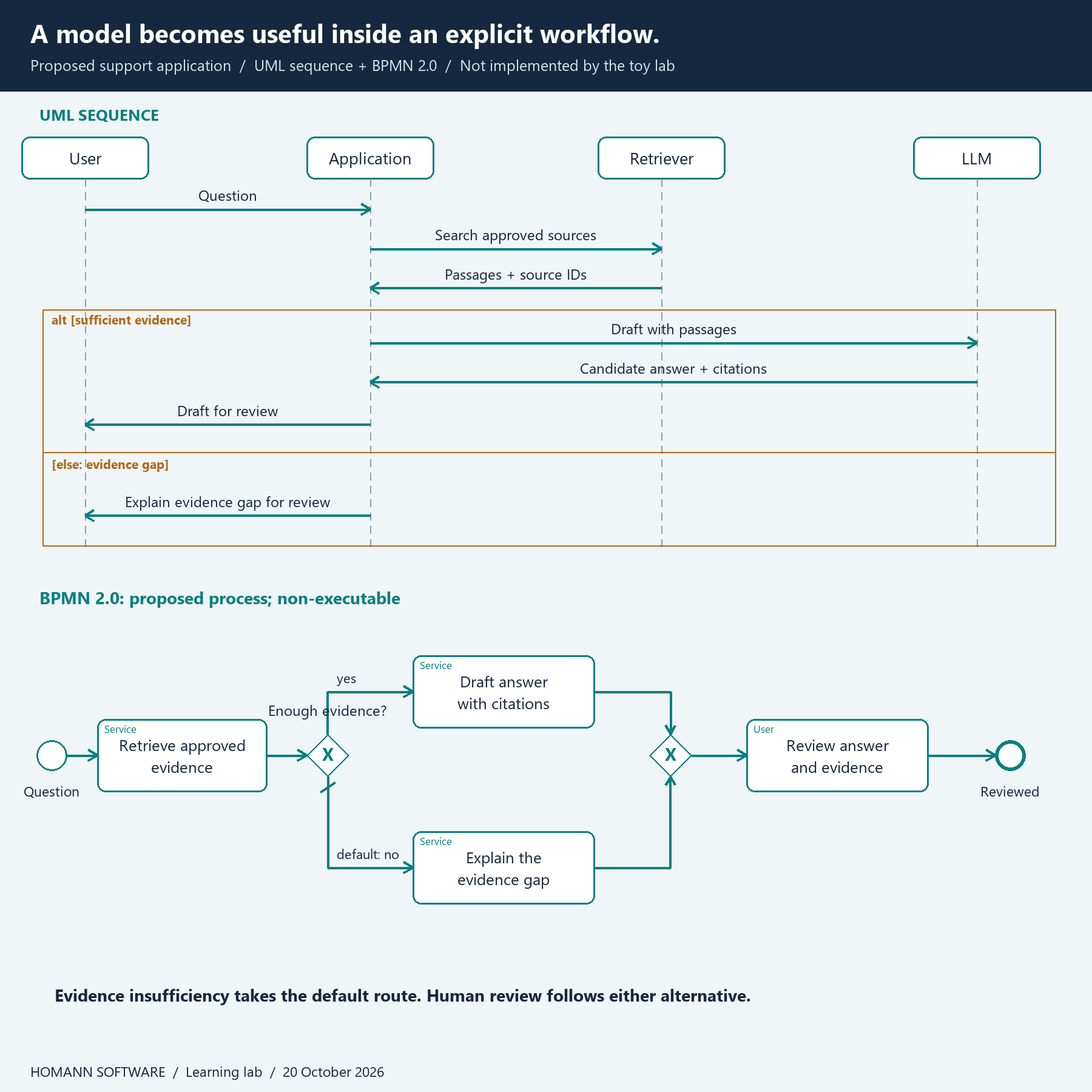
Figure 6. Two views of the same proposed support application. UML shows interactions; BPMN shows process control. Neither diagram claims that the toy Python code implements this application.
The UML sequence diagram describes who talks to whom and in what order. Its alternative fragment distinguishes enough evidence from an evidence gap. The BPMN 2.0 process describes business flow: a start event, retrieval, an exclusive evidence gateway, alternative drafting or gap-reporting tasks, an explicit merge, human review and an end event. It includes a default route for insufficient evidence.
The package includes editable PlantUML and a BPMN 2.0 XML file with diagram coordinates. The BPMN notation follows the OMG specification. It is a non-executable educational proposal, validated against the official XML schemas. No workflow engine, retrieval service, hosted LLM or production support application was executed as part of this article.
This system perspective connects with our MCP beginner guide: connecting a model to a capability is an integration concern. It does not alter the underlying distinction between training a model and invoking it.
17. Running and testing the learning lab
The examples were executed on Windows using Python 3.12.14, with no third-party runtime dependencies for the reader's experiments. Save the two complete files above together. The toolkit also contains test_examples.py and reproduction instructions.
Download the learning toolkit for the two modules, all tests, editable diagrams, research notes and execution evidence.
From that directory, run:
python neural_net.py
python language_lab.py
python -m unittest -v test_examples
All 26 tests passed. They include a numerical check of all 17 neural-network gradients, XOR fitting, stable loss at extreme logits, probability normalisation, invariance to a constant logit shift, the effect of temperature, known attention values, causal isolation, shape validation, smoothed bigram probabilities and non-mutating lookups.
The test count refers to 26 test methods; the parameter-by-parameter gradient checks are subtests within one method. This is not 26 model benchmarks. The runnable code teaches mechanisms, and the diagrams propose a possible application around a model.
Try three small changes. Increase or decrease the learning rate and observe loss. Change the bigram corpus and inspect the probabilities. Modify the future value vector and confirm that the first attention output is unchanged. Keep a record of the change and its result before drawing a conclusion.
18. A practical learning path
Start with the arithmetic of one prediction and one loss. Work through the XOR truth table, then trace one hidden unit's forward calculation in the supplied code. Run the network before changing its settings.
Next, investigate data and evaluation. Design a realistic split for a problem you understand. Write down what information exists at prediction time. Build a simple baseline, then compare a more flexible model under the same conditions. Explain the costs of false positives and false negatives before selecting a threshold.
Then move to language. Inspect tokenisation in a chosen model's own tooling rather than relying on word-count rules. Understand conditional probabilities, embedding vectors and the causal mask. Only then combine a model with retrieved evidence and an application workflow.
Finally, run a small task-specific evaluation on realistic cases. Record the model version, instructions, reference data and scoring rules. Include a question the system should decline to answer from insufficient evidence. For a business application, the ability to report an evidence gap can be more valuable than an extra paragraph of plausible prose.
19. What is changing now? A research snapshot for October 2026
The basics above help interpret several current developments. The following is a selected research snapshot, not a complete market ranking or a claim that any one product is universally best.
More attention to verification around models. Google Research's 14 October 2026 Deep Review announcement describes a document-review system that segments documents, allocates reasoning effort, performs specialised checks and synthesises grounded feedback. That is a reported system design from its developer. It illustrates a move toward verification workflows around a model; it is not independent proof that automated reviews are always correct. For beginners, the architectural lesson is that one model response and an evaluated multi-step application are different objects.
Efficiency can come from changing the task implementation. Google's 15 September 2026 Retrieve-for-Train research report describes compiling reward-optimised retrieval behaviour into a lightweight diffusion retriever. Its authors report faster inference in their evaluated search settings. Those task-specific findings do not establish an equivalent speedup for arbitrary chatbots. They show why training, distillation, retrieval and inference cost belong in the same engineering discussion.
AI systems increasingly combine modalities and specialised tools. Google's 14 October 2026 research overview covers systems involving geospatial models, scientific assistance and multimodal information. Text is one interface among several. The engineering implication is to evaluate the actual inputs, outputs and tool interactions of an application, rather than assuming that a text-only demo establishes performance with images, audio or sensor data.
Evaluation is struggling to keep pace with capability and adoption. The 2026 Stanford AI Index highlights a growing gap between AI capabilities and the institutions and methods used to govern, evaluate and understand them. This supports investing in measurement, while offering no shortcut to evidence for an individual deployment.
For Homann Software's architecture and engineering focus, the strongest editorial theme connecting these developments is understanding the learned model well enough to design and verify the system around it. That is our synthesis of the selected sources, not a ranking published by Stanford or Google. It is why this introduction spends as much care on data, evaluation and responsibility boundaries as on the network itself.
20. Technical metrics of leading model families
Snapshot checked on 20 October 2026. This is a selection of flagship and technically informative open-weight models from eight major providers, not an overall quality ranking. A provider's newest release is not necessarily its best option for every task. The figures below come from the linked model documentation and research reports; we did not benchmark these commercial models ourselves.
Read the units before comparing the numbers
One billion parameters is written as 1B; one trillion is 1T, or 1,000B. These are counts of learned numerical values, not neurons, training examples or context tokens. Our XOR network has 17 parameters; a model with 816B parameters operates at a vastly different scale.
In a dense network, most of the relevant model weights participate in each token's computation. A mixture-of-experts (MoE) network routes a token through selected expert blocks, alongside shared computation. The total parameter count and the active parameter count therefore answer different questions. Active parameters are not a direct measurement of latency, FLOPs or peak memory: attention, routing, communication, precision, batching and the serving hardware also matter.
NR means “not reported in the linked source reviewed for this snapshot.” It does not mean zero. In particular, we do not fill gaps in proprietary-model parameter counts with rumours or reverse-engineered estimates. Parameter-count scope also matters: a language backbone, a vision encoder and additional embedding tables are not automatically included in the same reported figure.
On a small screen, scroll the comparison tables sideways to see all columns.
Published parameter counts and access
| Model / provider | Published parameter counts | Active parameters per token | Architecture / access at the snapshot |
|---|---|---|---|
| OpenAI GPT-6 Astra | NR | NR | Hosted API; internal size not specified on the model page |
| OpenAI GPT-6.1 Sol | NR | NR | Hosted API; internal size not specified on the model page |
| Anthropic Claude Fable 5.1 | NR | NR | Hosted; demanding reasoning and agentic work |
| Anthropic Claude Opus 5.5 | NR | NR | Hosted; coding and knowledge work |
| Google Gemini 4 Argon | NR | NR | Sparse MoE Transformer; hosted |
| xAI / SpaceXSI Grok 4.7 | NR | NR | Hosted; numerical architecture details NR |
| Meta Muse Wonder / Wonder Full | NR | NR | Wonder: API and Muse Code; Full: Muse Code subscription |
| Meta Muse Spark Open | 816B total | 42B | MoE Transformer with perception encoder; downloadable weights under Muse Model License |
| Mistral Large 4 | 1.05T; a 1.6B vision encoder is also reported | 52B | Granular MoE; public API preview; weight release announced for month-end |
| DeepSeek V4.1-Flash | 552B backbone plus 196B Engram table parameters | 8B during prefill; 16B during decode | Causal encoder–decoder MoE; API and published checkpoints |
| Alibaba Qwen3.8-Max, cloud service | Based on the open model below; separate served-model total NR | Separate served-model count NR | Hosted version adds features beyond the released checkpoint |
| Alibaba Qwen3.8-2.4T-A95B, open checkpoint | 2.4T language-model parameters | 95B | Hybrid attention / MoE; downloadable weights under Qwen3.8-Max license |
Meta's open Spark model and its hosted Wonder models are separate entries; Spark's published parameter count must not be assigned to Wonder. Similarly, the Qwen model card identifies the cloud service as a version based on the open checkpoint, with additional features. We retain that distinction rather than asserting that every deployed component has the same parameter count.
Mistral's 6 October launch announcement says weights will follow by the end of the month. Calling a model “open-weight” in a preview announcement is not evidence that the weights were already downloadable on 20 October. The table uses the more specific 1.05T figure from its model documentation and does not silently add or subtract the separately listed vision encoder.
DeepSeek's architecture illustrates why one headline number can be incomplete: its technical report distinguishes backbone weights from Engram embedding tables, and distinguishes processing the input prefix, called prefill, from generating subsequent tokens, called decode. Its 8B and 16B figures refer to those different phases. The current API table identifies deepseek-flash as V4.1-Flash-1017. Historical V4-Pro figures should not be used to describe that endpoint; the launch announcement and the current API table differ about continued Pro routing, so we identify the Flash version explicitly.
Context windows, output limits and modalities
Context capacity is not model size. A context window limits how much tokenised material an invocation can work with; an output cap limits what it can emit. The input, output, internal reasoning and other overhead must fit the applicable limits. Do not add a maximum context figure and a maximum output figure to invent a larger usable window.
| Model / endpoint | Context window as documented | Separate output limit as documented | Inputs → outputs |
|---|---|---|---|
| GPT-6 Astra | 1,050,000 tokens | 128,000 tokens | Text, images → text |
| GPT-6.1 Sol | 1,050,000 tokens | 128,000 tokens | Text, images → text |
| Claude Fable 5.1 / Opus 5.5 | 1M tokens | 128K tokens | Text, images → text |
| Gemini 4 Argon | Up to 1M combined input + output | Separate generation cap NR in this model card | Text, images, audio, video → text |
| Grok 4.7 | 500,000 tokens | NR on this model page | Text, images → text |
| Muse Wonder / Wonder Full | 1M tokens | NR on this page | Modalities not specified in the cited specification table |
| Muse Spark Open | 1M at inference | Separate cap NR in its overview | Text, images, audio, video → text |
| Mistral Large 4 | 1M tokens | NR on this page | Multimodal input → generated text; preview features vary by endpoint |
| DeepSeek V4.1-Flash-1017 | 1M tokens | Maximum 384K tokens | Text, images → text |
| Qwen3.8-Max cloud | 1M tokens | 131K output; 262K reasoning is listed separately | Text, images → text |
| Qwen3.8-2.4T-A95B open checkpoint | 262,144 native; extensible to 1,010,000 | Framework-dependent; generation settings are not a universal API limit | Text → text; cloud-only vision features are not assumed |
We preserve the providers' K/M notation where they use it; these abbreviations should not be interpreted as an exact binary count unless the source supplies one. Limits may also depend on the platform, model version and reasoning configuration. A million-token context does not imply reliable recall of every supplied detail, and multimodal input support does not imply image or audio generation. An application with voice or video features may combine several models.
A closer look at two disclosed architectures
The Meta model card and Qwen model card also expose internal dimensions that help connect the large models with the small networks earlier in this guide:
| Model | LM layers | Hidden dimension | Expert routing | Vocabulary / embedding rows |
|---|---|---|---|---|
| Muse Spark Open | 62 | 8,192 | 256 experts; 8 activated per token | 202,048 |
| Qwen3.8-2.4T-A95B | 92 | 8,192 | 512 experts; 10 routed + 1 shared activated | 248,320, padded |
A hidden dimension of 8,192 means the model represents a token position with a vector of that width at the relevant backbone interfaces. It is not the model's parameter count. A layer contains multiple parameterised operations; vocabulary embeddings, attention projections and expert networks all contribute to the total. Expert counts describe routing structure, not 256 or 512 independent chatbots voting on an answer. These layer counts refer to the language backbone, not additional perception-encoder layers.
One explicit training-data disclosure is DeepSeek's reported 45T-token pretraining corpus for V4.1-Flash. That is a count of training tokens, not 45 trillion parameters or 45 trillion distinct documents. Tokenisation and modality encoding affect what such a budget represents; we do not invent matching training-data totals for the other models.
What parameter counts imply for memory
A deliberately simplified storage calculation is: number of parameters × bits per parameter ÷ 8. A hypothetical 100B-parameter model would require 200GB for 16-bit weights or 50GB for 4-bit weights, before any overhead. Those are decimal bytes and arithmetic examples, not measurements of a deployable model.
Actual inference also needs memory for attention state, often called the KV cache, activations, runtime buffers, quantisation metadata and other components. Long contexts and concurrent requests can increase that demand. MoE routing reduces the weights used for a particular token, but it does not make all other expert weights disappear from the deployment's storage requirements. Offloading and distributed serving change where those weights live. Training adds further requirements, including gradients and optimiser state. Parameter counts alone are therefore insufficient for choosing hardware or estimating a service's speed.
The practical comparison is task-specific: evaluate answer quality, unsupported claims, tool success, time to first token, generated tokens per second and cost per accepted outcome under matched conditions. The tables above provide technical specifications, not a benchmark leaderboard. No missing training-token count, training cost or private architecture detail is inferred from a model's name, price or fluent behaviour.
21. Questions beginners often ask
Does every AI system learn?
No. A rule engine or search algorithm can be part of AI without fitting parameters from data. A larger application can combine rules with learned models.
Does a chatbot learn from me during the conversation?
It can adapt its response to the supplied context without changing its trained weights. Saving conversation state, remembering information externally and later training on permitted data are separate mechanisms. Check the actual application's behaviour and terms.
Is an LLM a database or search engine?
A language model is a learned probability model. It can retain factual associations and sometimes memorise training material, but its ordinary generation path does not provide the guarantees of a database lookup. An application can add search or database tools.
Does a larger model always give a better answer?
No universal ordering follows from size. The task, data, training, context, tools and evaluation conditions matter. Compare systems on the job you need them to perform.
Are neural networks conscious or do they understand like people?
Producing useful language or passing a benchmark does not establish subjective experience. “Understanding” can refer to observable task ability or a stronger philosophical claim. Be clear which meaning you intend, and avoid treating fluent first-person text as evidence of consciousness.
Do I need a GPU to begin?
No. The supplied experiments run on a CPU. Training large models has very different resource requirements from learning these mechanisms or using a hosted inference service.
What should I remember first?
Training adjusts parameters using an objective and data. Inference applies the fitted model to inputs. Useful deployment requires evidence about the complete application. Once those three ideas are clear, neural networks and LLMs become much easier to reason about.